Anyone who has worked in Excel and used Tables knows how useful they are. And if you’ve worked in Excel but never used them, it’s time to start. Automatic expansion / shrinking, structured references, formulas or formatting propagating when you add new rows, using them as a source for charts, PivotTable or PowerQuery, easy and consistent filtering / sorting are just a few of the advantages. The only downside is that you can’t create subtotals.
Unfortunately, the Excel-equivalent app in the LibreOffice suite, Calc, doesn’t offer this feature. Let’s see how much we can “steal” from His Majesty, Microsoft.
In this article we’ll manually create a table, we’ll see what the differences are compared to an Excel table (what we lose), and in a future article we’ll automate everything, using an interface and code. Lots of code. Don’t worry, you’ll get everything spoon-fed 😀.
Some theoretical considerations
In Excel, a Table is, first of all, a combination of several well-defined cell regions that can each be accessed independently, and on them (or against them) you can perform various read, write, calculation, or formatting operations.
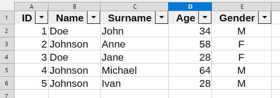
Assuming we have a table named Staff and the columns ID, Name, Surname, Age and Gender, these regions (Ranges) are the following:
| Area | Explanation | How to access |
|---|---|---|
| Table | The entire table, with everything related to it | Staff |
| Table header | Table first row | Staff[#Headers] |
| Totals | The last row of the table, contains the results of various calculations on columns (sums, averages…) | Staff[#Totals] |
| Data | The entire table from which we remove the table header and the totals row. | Staff[#Data] |
| “Name” column | The entire “Name” column | Staff[[#All],[Name]] |
| Data from “Name” column | The entire “Name” column, from which we remove the table header and the totals row. | Staff[[#Data],[Name]] |
For example, if we want to find out how many women are in the company, we use the formula:
=COUNTIF(Staff[[#Data],[Gender]];”F”)
instead of the formula
=COUNTIF(E$2:E$6;”F”)
This way we’re sure that no matter how much the column grows or shrinks vertically, the result stays consistent.
How to create a table in LibreOffice Calc
As I said at the beginning, we won’t be able to implement all the features. We’ll work with dynamic Named Ranges. Meaning they’ll update dynamically when we add or delete columns or rows.
What are Named Ranges? We’ve had them in Excel for many years as well. As the name suggests, they are regions of cells in a spreadsheet to which we assign a name. This makes them much easier to use in formulas. It’s easier and more “human” to write
=SUM(Quantity)
than
=SUM($C$121:$D$324)
On top of that, if I want the Quantity region to refer to another cell area, I only change the definition and the change is reflected in all results obtained based on Quantity.
To begin with, we create 2 ranges, LastRow and LastColumn. These will return the row number of the last row and the column number of the last column in the table. Yes, Named Ranges can also return values, not just cell areas.
We’ll assume the table is on the sheet named Sheet1.
- Go to the Sheet – Named Ranges and Expressions – Define… menu
- In Name type LastRow
- In Range or formula expression type the formula below
- In Scope choose Document (Global)
LOOKUP(2;1/($Sheet1.$A$2:$A$1048576<>””);ROW($Sheet1.$A$2:$A$1048576))
For LastColumn we proceed the same way, only the formula changes
LOOKUP(2;1/($Sheet1.$1:$1<>””);COLUMN($Sheet1.$1:$1))
For the entire table, same as above, but we name it Staff and in the formula we enter:
$Sheet1.$A$1:INDEX($Sheet1.$A:$XFD;LastRow;LastColumn)
Next, if we want to do something with the data in the Gender column, we’ll create the GenderData range, with the formula
$Sheet1.$E$2:INDEX($Sheet1.$E:$E;LastRow)
How to use what we’ve built
If we want to find out how many women are in the company, we’ll use the formula
=COUNTIF(GenderData;”F”)
A very useful feature in Excel tables is calculated columns. Meaning columns where each cell contains values calculated based on data from other columns on the same row.
To get in one column the value from another column, on the same row, we use the formula
INDEX(GenderData;ROW()-1)
Or, to be more correct (and to write more 😀)
INDEX(GenderData;ROW()-ROW(Staff))
because that 1 is actually the row number where the table starts (the row number where the table header is). See also FAQ no. 4 for why it’s better to use the second variant.
What to keep in mind. Tips and tricks
- The formulas above assume that the table starts in cell A1 and the data starts in cell A2.
- The formulas determine the size of the table by searching from A1 through the rest of the sheet. That’s 17,179,869,184 cells. The advantage is that I don’t have to worry when I add rows and columns. The disadvantages are the following:
- I can only have one table on the sheet
- Even though I haven’t used any volatile functions in the formulas, anything I write / modify / delete outside the table triggers a recalculation of all formulas
- The solution is to reserve a certain number of columns and rows for the table. In other words, the definition formulas only deal with the reserved area. This way I can use all the unreserved space. For other tables or anything else. My advice is to format that reserved area with an outer border. This way you’ll easily see when you’ve reached its edges and you can redo the reservation if needed.
- The solution works even if there are unfilled cells inside the table, including in the header (although why wouldn’t you fill in all the cells there?). Basically, the logic is as follows:
- For LastColumn, the formula starts from the first cell (A1 in our case) and goes to the right up to the last column of the sheet, keeping track of the last filled cell on the header row
- For LastRow, the formula starts from the first data cell of the table (A2 in our case) and searches down to the last cell of the sheet, keeping track of the last filled cell in the first column of the table
- Then, the entire Staff table is created starting from the first cell A1, searching the whole sheet until it hits LastColumn and LastRow
- For everything to work correctly, the following must be true:
- for LastColumn – in the header row all cells must be filled (if I only add a column to the right but don’t fill in the header, it won’t be taken into account). Sure, it also works if only the last cell in the header is filled, but then that’s no longer a proper header!
- for LastRow – in the first column at least the last cell must be filled
Let’s see what all these formulas do, so we know what to change.
LastRow
LOOKUP(2;1/($Sheet1.$A$2:$A$1048576<>””);ROW($Sheet1.$A$2:$A$1048576))
$A$2 – the cell where the data starts. This is what I change if my table starts in a different cell than $A$1
$A$1048576 – the last cell in the sheet, in column A. This is what I change if my table starts in a different column than A or if I want to reserve fewer rows than up to row 1,048,576. If I want to reserve 10 rows, the formula is
LOOKUP(2;1/($Sheet1.$A$2:$A$10<>””);ROW($Sheet1.$A$2:$A$10))
LastColumn
LOOKUP(2;1/($Sheet1.$1:$1<>””);COLUMN($Sheet1.$1:$1))
$1:$1 – the header row. Here I change 1 to the row number where the table starts. Pay attention to the formula for getting values from other columns.
If I want to reserve fewer columns than the sheet has, say 10 columns, the formula becomes the one below, because J is the 10th column:
LOOKUP(2;1/($Sheet1.$A$1:$J$1<>””);COLUMN($Sheet1.$A$1:$J$1))
The Staff table
$Sheet1.$A$1:INDEX($Sheet1.$A:$XFD;LastRow;LastColumn)
$A$1 – the cell where the table starts
$A:$XFD – all columns in the sheet
If I’ve reserved 10 rows and 10 columns, the formula becomes
$Sheet1.$A$1:INDEX($Sheet1.$A$1:$J$10;LastRow;LastColumn)
Data in the Gender column
$Sheet1.$E$2:INDEX($Sheet1.$E:$E;LastRow)
$E$2 – the cell where the data in the Gender column starts
If I’ve reserved 10 rows, the formula becomes
$Sheet1.$E$2:INDEX($Sheet1.$E$1:$E$10;LastRow)
Tables in LibreOffice Calc – FAQ
1. What happens if I add a new column to the table?
If you add a column to the right of the last column for which you created a Named Range, nothing happens, everything works normally. Of course, if you fit into the reserved area
However, if you add it to the left, you have to redo the definition of all Named Ranges of the columns after the inserted one.
2. What happens if I add rows above the table?
If the coordinates of the cell where the table starts change, you will have to modify all Named Ranges, possibly analyzing whether you are not exceeding the reserved area.
3. What happens if I add a new column to the left of the table?
If the coordinates of the cell where the table starts change, you will have to modify all Named Ranges, possibly analyzing whether you are not exceeding the reserved area.
4. The coordinates of the starting cell have changed, I have recreated all the Named Ranges, but the formulas that get data from other columns no longer work.
There may be two problems here:
- In the Named Range definition all coordinates must be given with $ both in the column and in the row.. $A1 is not the same as $A$1. The correct one is $A$1
- In the formula in the table you may have originally used ROW()-1 (the table started on row 1) and now the table starts on row 3. Either change all the formulas in the table or use ROW()-ROW(table_name) from the beginning, where instead of table_name you put the real name. See here
5. Where do I find Named Ranges?
In the Sheet menu - Named Ranges and Expressions - Manage... or with the shortcut Ctrl+F3. Here you will find all the Named Ranges defined, either for tables or for others.
Attention! You will not find them in the list on the left of the Formula Bar. Those defined directly as ranges of cells appear there, ours are defined by formulas.
6. I have a lot of Named Ranges, not just the ones for tables. And for each table I have many more for columns. How can I find them faster in the list?
My advice is to use the following naming convention for everything related to a table. Let's say we start with the Staff table:
- Table: tblStaff
- The last column and the last row: tblStaff_LC and tblStaff_LR
- For any column we use tblStaff_ColumnName rule, for example tblStaff_Name or tblStaff_Geneder
Using this convention, you will clearly see which tables and each column / LC / LR for that table are. Of course if you have two Date columns, the ranges will need to be named tblStaff_Date1 and tblStaff_Date2.
7. What's the deal with Scope when defining a Named Range?
Scope can have two values:
- Document (Global) - it is visible in any sheet. That is, I can use it in formulas in any sheet in the file. That is why I chose this Scope in our solution
- Sheet (the sheet name appears in the list) - it is visible only in the sheet where it was created. So I will be able to use it in formulas only in that sheet
8. Can I use the same name for two tables?
LibreOffice Calc does not allow two Named Ranges with the same Scope to have the same name. But it does allow it if the Scope is different.
What happens if I am on a sheet where I have a Named Range with Scope that sheet (tblStaff), but there is another one, somewhere in the file, with the same name and Scope = Global? The one in the sheet, with Scope = Sheet, takes priority. If I write a formula that refers to tblStaff in this sheet, it will read the data from tblStaff from here.
The advice is not to use the same name, even if Calc allows you to.
9. What happens if I duplicate a spreadsheet?
Named Ranges will also be duplicated, with the same names and definitions, but they will be automatically given Scope to the new sheet. This means that any formula external to the table and that was in that sheet, if it referred to the table, will work correctly, but will take the data from the new table, duplicated with the sheet, not from the original one. Because, as I said above, it has priority.
10. I have a central file with tables, but I want to access the data in another file. Is it possible?
That is, you simulate a central database. Very nice, but not here. LibreOffice Calc does not offer the possibility to access Named Ranges from other files.
11. What happens if I change the name of the sheet where I have the table and all the Named Ranges?
If you change the sheet name, this change will automatically be reflected in all formulas.
12. I changed the sheet name from "Sheet1" to "My Table" before creating Named Ranges. After filling in $My Table... errors appear
When the sheet name has spaces, it is written between single quotes $'My table'
Advantages and disadvantages of the solution
Pros
- The table expands / shrinks automatically
- No volatile functions are used in the formulas. Volatile functions are those that recalculate automatically on any change, anywhere in the file, even if I modify a cell that doesn’t depend on them. In large files that’s a disaster
- I can use calculated columns
Cons
- We don’t have a totals row
- Formulas in calculated columns don’t auto-copy down the column
- Formatting isn’t preserved when adding a new row
- There are no styles available to format the entire table
- If I move the table somewhere else on the sheet or to another sheet, all functionality is lost and all Named Ranges have to be recreated
What’s next?
Nice things, what else? Maybe to visually create tables?
Until then,
Happy Coding!
Sources: featured image created with AI ChatGPT